Flow Inversion

This section is an example of solving the flow equation with the Newton-Raphson method. The governing equations are derived from conservation of mass of each phase, and conservation of momentum or Darcy's law for each phase. First, we have

\[\frac{\partial }{{\partial t}}(\phi {S_i}{\rho _i}) + \nabla \cdot ({\rho _i}{\mathbf{v}_i}) = {\rho _i}{q_i}, \quad i = 1,2 \tag{1}\]

The saturation of the two phases satisfies

\[S_{1} + S_{2} = 1\tag{2}\]

and the Darcy's law yields

\[{\mathbf{v}_i} = - \frac{{K{k_{ri}(S_i)}}}{{{\tilde{\mu}_i}}}(\nabla {P_i} - g{\rho _i}\nabla Z), \quad i=1,2 \tag{3}\]

Here, $K$ is the permeability tensor, but in our case we assume it is a space varying scalar value. $k_{ri}(S_i)$ is a function of $S_i$, and typically the higher the saturation, the easier the corresponding phase is to flow. $\tilde \mu_i$ is the viscosity ^[pcl]. $Z$ is the depth cordinate, $\rho_i$ is the density, $\phi$ is the porosity, $q_i$ is the source, $P_i$ is the fluid pressure and $g$ is the velocity constant.

The fluid pressure $P_i$ is related to $S_i$ via the capillary pressure

\[P_2 = P_1 - P_c(S_2)\tag{4}\]

where $P_c$ is a function of the saturation of the wetting phase 2.

In Equations 1-4, the state variables are $S_1$, $S_2$, $\mathbf{v}_i$, $P_1$, and $P_2$. There are 6 equations and 6 variables (taking dimension into consideration) in total, and thus the system is complete.

Info

In all the numerical scheme below, we adopt the finite volumn method. Each cell in the following discretized domain is a cell and the state variables $\Psi_2, S_1, S_2$ and the capillary potential $\Psi_c$ are defined per cell.

Step 1: Parameters Setup

const K_CONST =  9.869232667160130e-16 * 86400 * 1e3
const ALPHA = 1.0
mutable struct Ctx
  m; n; h; NT; Δt; Z; X; ρw; ρo;
  μw; μo; K; g; ϕ; qw; qo; sw0
end

function tfCtxGen(m,n,h,NT,Δt,Z,X,ρw,ρo,μw,μo,K,g,ϕ,qw,qo,sw0,ifTrue)
  tf_h = constant(h)
  # tf_NT = constant(NT)
  tf_Δt = constant(Δt)
  tf_Z = constant(Z)
  tf_X= constant(X)
  tf_ρw = constant(ρw)
  tf_ρo = constant(ρo)
  tf_μw = constant(μw)
  tf_μo = constant(μo)
  # tf_K = isa(K,Array) ? Variable(K) : K
  if ifTrue
    tf_K = constant(K)
  else
    tf_K = Variable(K)
  end
  tf_g = constant(g)
  # tf_ϕ = Variable(ϕ)
  tf_ϕ = constant(ϕ)
  tf_qw = constant(qw)
  tf_qo = constant(qo)
  tf_sw0 = constant(sw0)
  return Ctx(m,n,tf_h,NT,tf_Δt,tf_Z,tf_X,tf_ρw,tf_ρo,tf_μw,tf_μo,tf_K,tf_g,tf_ϕ,tf_qw,tf_qo,tf_sw0)
end

function Krw(Sw)
    return Sw ^ 1.5
end

function Kro(So)
    return So ^1.5
end

function ave_normal(quantity, m, n)
    aa = sum(quantity)
    return aa/(m*n)
end

Step 2: Implementing the Numerical Scheme

The major simulation codes consist of using a nonlinear implicit timestep for (1),

\[\phi (S_2^{n + 1} - S_2^n) - \nabla \cdot \left( {{m_{2}}(S_2^{n + 1})K\nabla \Psi _2^n} \right) \Delta t = \left(q_2^n + q_1^n \frac{m_2(S^{n+1}_2)}{m_1(S^{n+1}_2)}\right) \Delta t \tag{5}\]

Here $m_i(s) = \frac{k_{ri}(s)}{\tilde \mu_i}$ and $\Psi_i = P_i - \rho_i g Z$.

In sat_op we solve the nonlinear equation (5) with a Newton-Raphson scheme.

# variables : sw, u, v, p
# (time dependent) parameters: qw, qo, ϕ
function onestep(sw, p, m, n, h, Δt, Z, ρw, ρo, μw, μo, K, g, ϕ, qw, qo)
    # step 1: update p
    # λw = Krw(sw)/μw
    # λo = Kro(1-sw)/μo
    λw = sw.*sw/μw
    λo = (1-sw).*(1-sw)/μo
    λ = λw + λo
    q = qw + qo + λw/(λo+1e-16).*qo
    # q = qw + qo
    potential_c = (ρw - ρo)*g .* Z

    # Step 1: implicit potential
    Θ = upwlap_op(K * K_CONST, λo, potential_c, h, constant(0.0))

    load_normal = (Θ+q/ALPHA) - ave_normal(Θ+q/ALPHA, m, n)

    # p = poisson_op(λ.*K* K_CONST, load_normal, h, constant(0.0), constant(1))
    p = upwps_op(K * K_CONST, λ, load_normal, p, h, constant(0.0), constant(0)) # potential p = pw - ρw*g*h 

    # step 2: implicit transport
    sw = sat_op(sw, p, K * K_CONST, ϕ, qw, qo, μw, μo, sw, Δt, h)
    return sw, p
end


function imseq(tf_ctx)
    ta_sw, ta_p = TensorArray(NT+1), TensorArray(NT+1)
    ta_sw = write(ta_sw, 1, tf_ctx.sw0)
    ta_p = write(ta_p, 1, constant(zeros(tf_ctx.m, tf_ctx.n)))
    i = constant(1, dtype=Int32)
    function condition(i, tas...)
        i <= tf_ctx.NT
    end
    function body(i, tas...)
        ta_sw, ta_p = tas
        sw, p = onestep(read(ta_sw, i), read(ta_p, i), tf_ctx.m, tf_ctx.n, tf_ctx.h, tf_ctx.Δt, tf_ctx.Z, tf_ctx.ρw, tf_ctx.ρo, tf_ctx.μw, tf_ctx.μo, tf_ctx.K, tf_ctx.g, tf_ctx.ϕ, tf_ctx.qw[i], tf_ctx.qo[i])
        ta_sw = write(ta_sw, i+1, sw)
        ta_p = write(ta_p, i+1, p)
        i+1, ta_sw, ta_p
    end

    _, ta_sw, ta_p = while_loop(condition, body, [i, ta_sw, ta_p])
    out_sw, out_p = stack(ta_sw), stack(ta_p)
end

Step 3: Forward Computation

We now first generate the synthetic data.

using FwiFlow
using PyCall
using LinearAlgebra
using DelimitedFiles
np = pyimport("numpy")

const SRC_CONST = 86400.0 #
const GRAV_CONST = 9.8    # gravity constant

# Hyperparameter for flow simulation
m = 15
n = 30
h = 30.0 # meter
NT  = 50
dt_survey = 5
Δt = 20.0 # day
z = (1:m)*h|>collect
x = (1:n)*h|>collect
X, Z = np.meshgrid(x, z)

ρw = 501.9
ρo = 1053.0
μw = 0.1
μo = 1.0

K_init = 20.0 .* ones(m,n) # initial guess of permeability 

g = GRAV_CONST
ϕ = 0.25 .* ones(m,n)
qw = zeros(NT, m, n)
qw[:,9,3] .= 0.005 * (1/h^2)/10.0 * SRC_CONST
qo = zeros(NT, m, n)
qo[:,9,28] .= -0.005 * (1/h^2)/10.0 * SRC_CONST
sw0 = zeros(m, n)
survey_indices = collect(1:dt_survey:NT+1) # 10 stages
n_survey = length(survey_indices)



K = 20.0 .* ones(m,n) # millidarcy
K[8:10,:] .= 120.0
tfCtxTrue = tfCtxGen(m,n,h,NT,Δt,Z,X,ρw,ρo,μw,μo,K,g,ϕ,qw,qo, sw0, true)
out_sw_true, out_p_true = imseq(tfCtxTrue)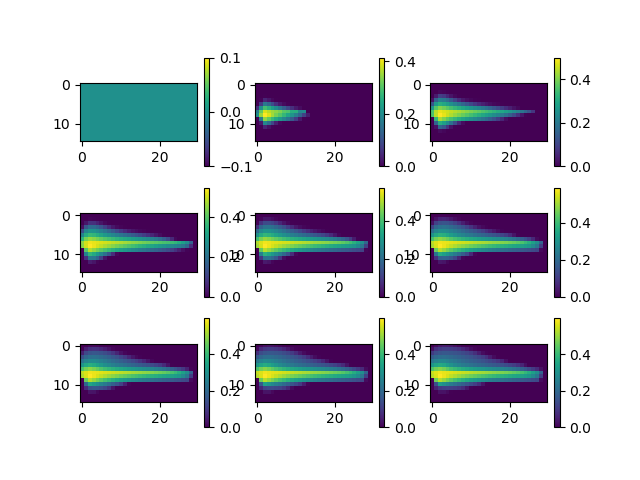

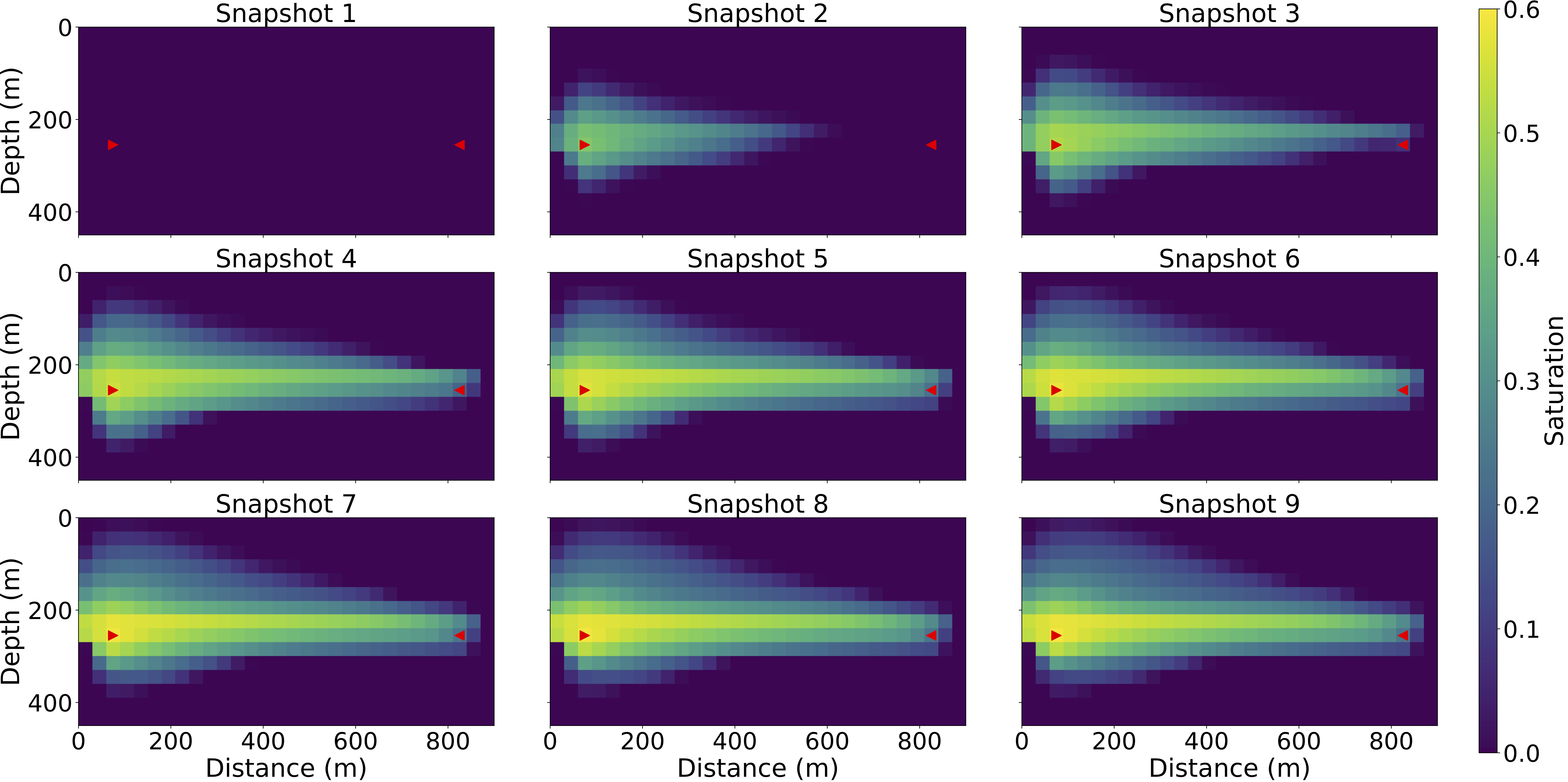
Step 4: Inversion

We now conduct inversion. The unknown variable is stored in tfCtxInit.K.

tfCtxInit = tfCtxGen(m,n,h,NT,Δt,Z,X,ρw,ρo,μw,μo,K_init,g,ϕ,qw,qo, sw0, false)
out_sw_init, out_p_init = imseq(tfCtxInit)

sess = Session(); init(sess)
O = run(sess, out_sw_init)
vis(O)
# NOTE Compute FWI loss


loss = sum((out_sw_true-out_sw_init)^2)
opt = ScipyOptimizerInterface(loss, options=Dict("maxiter"=> 100, "ftol"=>1e-12, "gtol"=>1e-12),var_to_bounds = Dict(tfCtxInit.K=>(10.0, 130.0)))
       

__cnt = 0
__loss = 0
out = []
function print_loss(l)
    if mod(__cnt,1)==0
        println("iter $__cnt, current loss=",l)
    end
    global __loss = l
    global __cnt += 1
end
__iter = 0
function step_callback(rk)
    if mod(__iter,1)==0
        println("================ ITER $__iter ===============")
    end
    println("$__loss")
    push!(out, __loss)
    global __iter += 1
end
sess = Session(); init(sess)
ScipyOptimizerMinimize(sess, opt, loss_callback=print_loss, 
        step_callback=step_callback, fetches=[loss])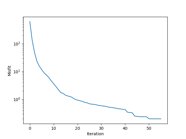

We can visualize K with

imshow(run(sess, tfCtxInit.K), extent=[0,n*h,m*h,0]);
xlabel("Distance (m)")
ylabel("Depth (m)")
cb = colorbar()
clim([20, 120])
cb.set_label("Permeability (md)")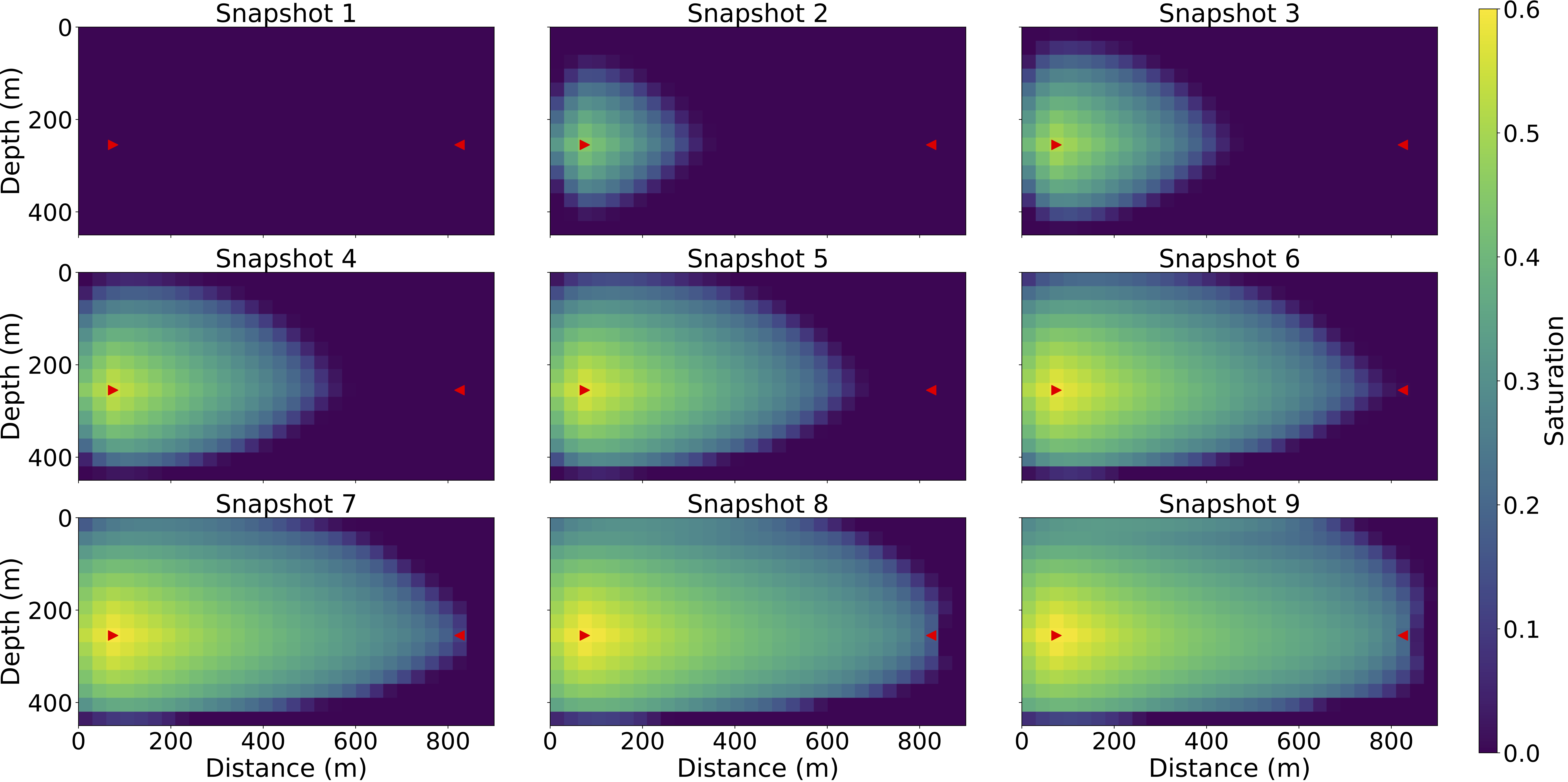

pcl This paper gives a description of common relative permeability models and proposes a method to calibrate an empirical model from indirect data.