Time Fractional Differential Equation

The fractional calculus has motivated development and application of novel algorithms and models for describing anomoulous diffusion. In this section, we discuss how to carry out numerical simulation of time fractional differential equations and the corresponding inversion. The major operator in FwiFlow is time_fractional_op and time_fractional_t_op.

We consider the function

\[u(t) = t^\beta\]

Then the corresponding time derivative is

\[D^\alpha_{t_0}u(t) = \frac{\Gamma(\beta+1)}{\Gamma(\beta-\alpha+1)} t^{\beta-\alpha}\]

using FwiFlow
Γ = x->exp(tf.math.lgamma(convert_to_tensor(x)))


function u(t, α)
  t^β
end
function du(t, α)
  Γ(β+1)/Γ(β-α+1)* t^(β-α)
end

β = 8.0
α = 0.8
NT = 100
f = (t, u, θ) -> du(t, α)
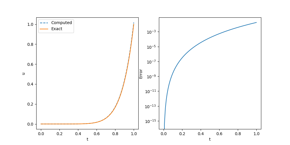
uout = time_fractional_op(α, f, 1.0, 0.0, NT)

sess = Session(); init(sess)
uval = run(sess, uout)

We can compare the exact solution and the numerical solution and they are nearly the same.

We can also measure the convergence order in terms of mean square error (MSE)

$\alpha=0.2$	Rate	$\alpha=0.5$	Rate	$\alpha=0.8$	Rate
7.1536E-04		3.4743E-03		1.1166E-02
2.2060E-04	1.70	1.2516E-03	1.47	4.7746E-03	1.23
6.7502E-05	1.71	4.5055E-04	1.47	2.0644E-03	1.21
2.0484E-05	1.72	1.6170E-04	1.48	8.9669E-04	1.20
6.1669E-06	1.73	5.7842E-05	1.48	3.9018E-04	1.20

Now we consider inverse modeling. In this problem, $\alpha$ is not know and we can only observe part of the solution. For example, we only know $u(2.0)$, initial conditions and the source function and we want to estimate $\alpha$. We can mark $\alpha$ as an independent variable for optimization by using Variable key word.

using FwiFlow
Γ = x->exp(tf.math.lgamma(convert_to_tensor(x)))

function u(t, α)
  t^β
end
function du(t, α)
  Γ(β+1)/Γ(β-α+1)* t^(β-α)
end

β = 8.0
α = Variable(0.5)
NT = 200
f = (t, u, θ) -> du(t, 0.8)
uout = time_fractional_op(α, f, 1.0, 0.0, NT)
loss = (uout[NT+1] - 1.0)^2

sess = Session(); init(sess)
opt = ScipyOptimizerInterface(loss, method="L-BFGS-B",options=Dict("maxiter"=> 100, "ftol"=>1e-12, "gtol"=>1e-12), var_to_bounds=Dict(α=>(0.0,1.0)))
ScipyOptimizerMinimize(sess, opt)
@show run(sess, α)

We have the estimation

\[\alpha = 0.8036829691152347\]